What Makes Multi-modal Learning Better than Single (Provably)
What Makes Multi-modal Learning Better than Single (Provably)
Introduction
우리 세상에는 시각, 청각, 텍스트 등 다양한 modality가 존재한다. 직관적으로 여러 modality의 정보를 결합(fusion)하면 하나만 사용하는 것보다 더 나은 성능을 얻을 수 있을 것이라 기대된다. 실제로 딥러닝에서도 RGB-D semantic segmentation, audio-visual learning, Visual Question Answering 등 multi-modal 학습이 활발히 연구되고 있으며, 경험적으로 좋은 성과를 보이고 있다.
하지만 이론적 근거는 부족했다. 기존 이론 연구들은 modality 간 확률 분포에 대한 강한 가정을 하거나, generalization 관점을 고려하지 않았다.
이 논문은 다음 두 가지 질문에 대해 이론적 증명과 실험적 검증을 제시한다.
- (When) 어떤 조건에서 multi-modal이 uni-modal보다 성능이 좋은가?
- (Why) multi-modal 학습이 더 나은 성능을 제공하는 이유는 무엇인가?
핵심 결론: multi-modal 학습의 이점은 더 정확한 latent space representation을 학습할 수 있기 때문이다. 다만 데이터가 충분히 많을 때라는 조건이 필요하다.
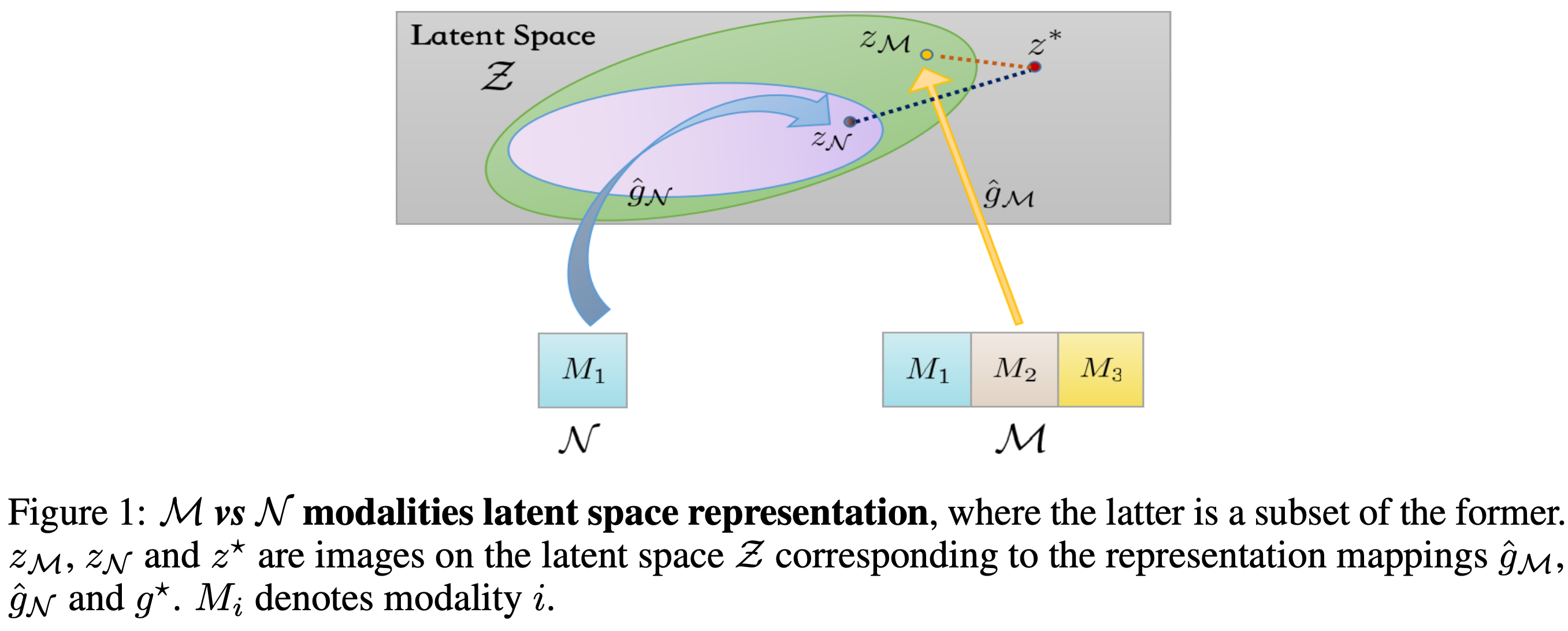
The Multi-modal Learning Formulation
데이터 정의
\(K\)개의 modality가 있다고 하자. 데이터는 다음과 같이 표현된다.
\[\mathbb{x} := (x^{(1)}, \cdots, x^{(K)}), \quad x^{(k)} \in \mathcal{X}^{(k)}\]전체 input space는 \(\mathcal{X} = \mathcal{X}^{(1)} \times \cdots \times \mathcal{X}^{(K)}\)이다.
이 논문에서 사용하는 composite multi-modal framework는 두 단계로 구성된다.
- Encoding: 여러 modality의 feature를 공통 latent space \(\mathcal{Z}\)로 매핑 — \(g^\star: \mathcal{X} \mapsto \mathcal{Z}\)
- Task mapping: Latent representation을 target space로 매핑 — \(h^\star: \mathcal{Z} \mapsto \mathcal{Y}\)
예를 들어, video classification에서 각 modality \(k\) (RGB, audio, optical flow)를 개별 네트워크 \(\varphi_k\)로 인코딩하고, fusion operation \(\oplus\)로 합친 뒤, classifier \(\mathcal{C}\)에 통과시키는 late-fusion 구조가 이에 해당한다.
\[g_\mathcal{M}(\mathbb{x}) = \varphi_1 \oplus \varphi_2 \oplus \cdots \oplus \varphi_M\]Subset Modalities
\(K\)개의 modality 중 subset \(\mathcal{M}\)만 사용할 수 있다. 사용하지 않는 modality는 \(\bot\)으로 표시한다.
\[p_\mathcal{M}(\mathbb{x})^{(k)} = \begin{cases} \mathbb{x}^{(k)} & \text{if } k \in \mathcal{M} \\ \bot & \text{else} \end{cases}\]핵심 질문: \(\mathcal{N} \subset \mathcal{M}\)일 때 (\(\mathcal{N}\)이 \(\mathcal{M}\)의 부분집합), 항상 \(\mathcal{M}\)으로 학습하는 것이 더 좋은가?
학습 목표: Empirical Risk Minimization
데이터셋 \(\mathcal{S} = \{(\mathbb{x}_i, y_i)\}_{i=1}^m\)에 대해, ERM으로 학습한다.
\[\min_{h \in \mathcal{H}, \, g_\mathcal{M} \in \mathcal{G}_\mathcal{M}} \hat{r}(h \circ g_\mathcal{M}) = \frac{1}{m} \sum_{i=1}^{m} \ell(h \circ g_\mathcal{M}(\mathbb{x}_i), y_i)\]Population risk는 이 empirical risk의 기댓값이다.
\[r(h \circ g_\mathcal{M}) = \mathbb{E}_{(\mathbb{x}_i, y_i) \sim \mathcal{D}}[\hat{r}(h \circ g_\mathcal{M})]\]Main Results
Latent Representation Quality
학습된 latent representation \(g\)가 true representation \(g^\star\)에 얼마나 가까운지를 측정하는 핵심 지표를 정의한다.
Definition 1. 학습된 latent representation mapping \(g \in \mathcal{G}\)의 latent representation quality는 다음과 같이 정의된다.
\[\eta(g) = \inf_{h \in \mathcal{H}} [r(h \circ g) - r(h^\star \circ g^\star)]\]
직관적으로, \(\eta(g)\)는 학습된 representation \(g\)를 사용했을 때 가장 좋은 경우에도 true representation 대비 얼마나 loss가 증가하는지를 측정한다. \(\eta(g) = 0\)이면 완벽한 representation이고, 클수록 나쁘다.
핵심 insight: Population risk의 차이가 latent representation quality의 차이에 의해 결정된다면, 더 나은 representation을 학습하는 것이 곧 더 나은 성능을 의미한다.
Rademacher Complexity
모델의 complexity를 측정하기 위해 Rademacher complexity를 사용한다. 함수 집합 \(\mathcal{F}\)와 sample \(S = (Z_1, \ldots, Z_m)\)에 대해:
\[\hat{\mathfrak{R}}_S(\mathcal{F}) := \mathbb{E}_\sigma \left[ \sup_{f \in \mathcal{F}} \frac{1}{m} \sum_{i=1}^{m} \sigma_i f(Z_i) \right]\]여기서 \(\sigma_i \sim \text{Uniform}\{-1, +1\}\)이다. Rademacher complexity가 높을수록 함수 집합이 복잡하여 overfitting 위험이 크다.
Theorem 1: Population Risk와 Latent Quality의 관계
Theorem 1. 데이터셋 \(S = \{(\mathbb{x}_i, y_i)\}_{i=1}^m\)이 분포 \(\mathcal{D}\)에서 i.i.d.로 추출되었다고 하자. \(\mathcal{M}, \mathcal{N}\)이 \([K]\)의 서로 다른 부분집합이고, 각각으로 학습한 ERM minimizer가 \((\hat{h}_\mathcal{M}, \hat{g}_\mathcal{M})\), \((\hat{h}_\mathcal{N}, \hat{g}_\mathcal{N})\)일 때, 확률 \(1 - \delta/2\) 이상으로:
\[r(\hat{h}_\mathcal{M} \circ \hat{g}_\mathcal{M}) - r(\hat{h}_\mathcal{N} \circ \hat{g}_\mathcal{N}) \leq \gamma_S(\mathcal{M}, \mathcal{N}) + 8L\mathfrak{R}_m(\mathcal{H} \circ \mathcal{G}_\mathcal{M}) + \frac{4C}{\sqrt{m}} + 2C\sqrt{\frac{2\ln(2/\delta)}{m}}\]여기서 \(\gamma_S(\mathcal{M}, \mathcal{N}) \triangleq \eta(\hat{g}_\mathcal{M}) - \eta(\hat{g}_\mathcal{N})\)는 latent representation quality의 차이이다.
이 정리가 말하는 것
우변의 항들을 분석하면:
- \(\gamma_S(\mathcal{M}, \mathcal{N})\): Latent representation quality의 차이. \(\mathcal{M}\)의 representation이 더 좋으면 음수가 되어 population risk가 줄어든다.
- \(8L\mathfrak{R}_m(\mathcal{H} \circ \mathcal{G}_\mathcal{M})\): 모델 복잡도. Modality가 많을수록 함수 공간이 커져서 이 항이 증가한다.
- \(O(1/\sqrt{m})\) 항들: 데이터 크기에 반비례. 데이터가 많으면 사라진다.
즉, 데이터가 충분히 많으면 (\(m\)이 크면) 2, 3번 항이 사라지고 latent representation quality만 남는다. 더 많은 modality가 더 좋은 representation을 제공하므로 multi-modal이 유리하다.
반대로 데이터가 적으면 2번 항(모델 복잡도)이 지배적이 되어, 오히려 modality 수를 줄이는 것이 나을 수 있다.
Theorem 2: Latent Quality의 Upper Bound
Theorem 2. \(\mathcal{M}\) modalities로 학습한 ERM minimizer \((\hat{h}_\mathcal{M}, \hat{g}_\mathcal{M})\)에 대해, 확률 \(1 - \delta\) 이상으로:
\[\eta(\hat{g}_\mathcal{M}) \leq 4L\mathfrak{R}_m(\mathcal{H} \circ \mathcal{G}) + 4\mathfrak{R}_m(\mathcal{H} \circ \mathcal{G}) + 6C\sqrt{\frac{2\ln(2/\delta)}{m}} + \hat{L}(\hat{h}_\mathcal{M} \circ \hat{g}_\mathcal{M}, S)\]
이 정리에서 중요한 관찰: \(\mathcal{N} \subset \mathcal{M}\)이면 \(\mathcal{G}_\mathcal{N} \subset \mathcal{G}_\mathcal{M} \subset \mathcal{G}\)이므로, \(\mathcal{N}\)의 function class가 더 작다. 따라서 centered empirical loss \(\hat{L}\)이 더 커질 수 있다. 이는 더 적은 modality로 학습하면 latent quality가 더 나빠질 수 있음을 의미한다.
Modality 선택 원칙
Theorem 2로부터 다음 원칙이 도출된다.
Principle: 더 많은 modality를 사용하는 것이 좋다. 단, 다음 조건을 만족해야 한다:
\[\hat{L}(\hat{h}_\mathcal{N} \circ \hat{g}_\mathcal{N}, S) - \hat{L}(\hat{h}_\mathcal{M} \circ \hat{g}_\mathcal{M}, S) \geq \sqrt{\frac{C(\mathcal{H} \circ \mathcal{G}_\mathcal{M})}{m}} - \sqrt{\frac{C(\mathcal{H} \circ \mathcal{G}_\mathcal{N})}{m}}\]
즉, (i) 데이터가 많으면 우변이 작아져서 거의 항상 multi-modal이 유리하고, (ii) 데이터가 적으면 function class complexity의 차이(우변)가 커져서 uni-modal이 나을 수 있다.
Proposition 1: Linear Model에서의 검증
Linear model (\(g(\mathbb{x}) = A^\top \mathbb{x}\), \(h(\mathbb{z}) = \beta^\top \mathbb{z}\))에서, 전체 modality \(\mathcal{M} = [K]\)와 하나를 뺀 \(\mathcal{N} = [K-1]\)에 대해:
\[\gamma_S(\mathcal{M}, \mathcal{N}) \leq 0\]이는 더 많은 modality를 사용하면 latent representation quality가 항상 같거나 더 좋다는 것을 직접 증명한다.
Experiment
실험은 실제 데이터셋과 합성 데이터셋으로 나누어 진행했다.
Real-world Dataset: IEMOCAP
데이터셋
Interactive Emotional Dyadic Motion Capture (IEMOCAP) 데이터베이스를 사용했다.
- Modalities: Text (100차원), Video (500차원), Audio (100차원)
- Task: 발화자의 감정 분류 (6개 클래스: happy, sad, neutral, angry, excited, frustrated)
- 데이터 크기: Training 13,200개, Testing 3,410개
학습 설정
- Encoder: 1개의 linear layer, hidden dimension 128
- 각 modality별 개별 encoder (weight 비공유)
- Late-fusion: 각 encoder 출력을 concatenation 후 task mapping
- Optimizer: Adam (lr=0.01), batch size: 2048
- Top-1 accuracy로 평가
결과 1: Modality 조합별 성능
| Modalities | Test Accuracy |
|---|---|
| Text (T) | 49.93 ± 0.57 |
| Text + Video (TV) | 51.08 ± 0.66 |
| Text + Audio (TA) | 53.03 ± 0.21 |
| Text + Video + Audio (TVA) | 53.89 ± 0.47 |
Modality가 많을수록 정확도가 향상된다. 특히 Audio가 추가되었을 때 가장 큰 폭의 향상이 있는데, 이는 감정 인식에서 음성 톤이 매우 중요한 정보를 제공하기 때문이다.
결과 2: Sample Size와 Modality의 관계
| Modalities | \(10^{-4}\) | \(10^{-3}\) | \(10^{-2}\) | \(10^{-1}\) | 1 (전체) |
|---|---|---|---|---|---|
| T | 23.66 | 29.08 | 45.63 | 48.30 | 49.93 |
| TA | 25.06 | 34.28 | 47.28 | 50.46 | 53.03 |
| TV | 24.71 | 38.37 | 46.54 | 49.50 | 51.08 |
| TVA | 24.71 | 32.24 | 46.39 | 50.75 | 53.89 |
핵심 관찰: 데이터가 충분할 때(비율 \(10^{-1}\) 이상)는 TVA가 최고 성능이다. 하지만 데이터가 매우 적을 때(\(10^{-4}\))는 TA(2개 modality)가 TVA(3개 modality)보다 오히려 높다.
이는 Theorem 1의 예측과 정확히 일치한다. 데이터가 적으면 function class complexity (\(\mathfrak{R}_m\)) 항이 지배적이 되어, 더 많은 modality가 오히려 overfitting을 유발한다.
결과 3: Latent Representation Quality 비교
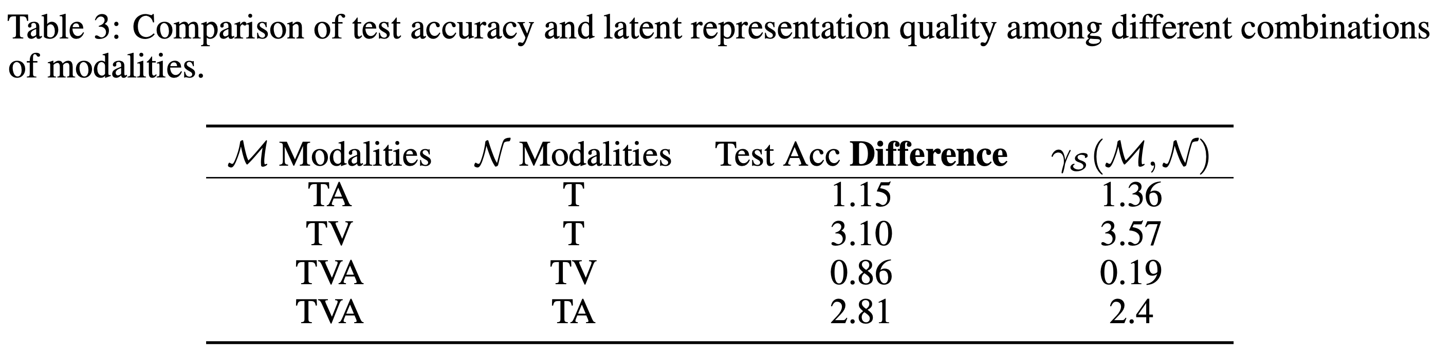
| \(\mathcal{M}\) | \(\mathcal{N}\) | Test Acc Difference | \(\gamma_S(\mathcal{M}, \mathcal{N})\) |
|---|---|---|---|
| TA | T | 1.15 | 1.36 |
| TV | T | 3.10 | 3.57 |
| TVA | TV | 0.86 | 0.19 |
| TVA | TA | 2.81 | 2.4 |
모든 경우에서 \(\gamma_S(\mathcal{M}, \mathcal{N}) > 0\)이다. 즉, 더 많은 modality를 사용할수록 latent representation quality가 더 좋고, 이것이 test accuracy 향상으로 이어진다. Test accuracy 차이와 \(\gamma_S\) 값이 같은 부호라는 것이 Theorem 1을 실험적으로 검증한다.
\(\eta(\hat{g}_\mathcal{M})\)는 다음과 같이 측정했다. Encoder \(\hat{g}_\mathcal{M}\)을 freeze한 후 classifier \(h\)만 fine-tuning하여 얻는 best population risk에서 oracle risk를 뺀 값이다.
Synthetic Data
합성 데이터로 modality 간 correlation의 영향을 분석했다. 4개의 modality \(m_1, m_2, m_3, m_4\)를 생성하되, overlap parameter \(w\)로 modality 간 정보 공유 정도를 조절한다.
- \(w = 1\): 모든 modality가 같은 정보 공유 (높은 상관)
- \(w = 0\): 각 modality가 완전히 독립적
| Modalities | \(w=1\) | \(w=0.8\) | \(w=0.5\) | \(w=0.2\) | \(w=0\) |
|---|---|---|---|---|---|
| \(m_1\) | 0 | 12.04 | 75.89 | 193.28 | 301.92 |
| \(m_1, m_2\) | 0 | 8.16 | 51.25 | 129.81 | 207.45 |
| \(m_1, m_2, m_3\) | 0 | 4.18 | 26.06 | 65.17 | 103.23 |
| \(m_1, m_2, m_3, m_4\) | 0 | 0 | 0 | 0 | 0 |
관찰: modality 수가 많을수록 MSE loss(\(\eta\))가 줄어든다. 또한 modality 간 상관이 높을수록(\(w\)가 클수록) 더 적은 modality로도 좋은 representation을 학습할 수 있다. 이는 Theorem 2의 예측과 일치한다.
Discussion
이 논문의 이론적 결과는 generalization 관점에서 multi-modal의 우위를 설명한다. 이는 optimization 관점의 기존 연구와 상호보완적이다.
실제로 multi-modal 학습이 항상 좋지는 않다는 관찰도 있다. Modality 간 interaction이 학습 과정에서 최적화 어려움을 유발할 수 있는데, 이는 이 논문의 이론적 framework에서는 다루지 않는 부분이다. 이 논문은 “최적화가 잘 된다고 가정할 때” multi-modal이 더 나은 generalization을 보장한다는 것을 증명한다.
Conclusion
- When: 데이터가 충분히 많고 function class complexity가 잘 통제될 때 multi-modal이 유리하다.
- Why: Multi-modal은 더 정확한 latent space representation을 학습할 수 있기 때문이다. 이는 latent representation quality \(\eta(g)\)로 형식화되며, population risk와 직접 연결된다.
- 이론적 분석(Theorem 1, 2)과 실험(IEMOCAP, 합성 데이터) 모두 이를 뒷받침한다.
- 다만 데이터가 적을 때는 modality 수를 줄이는 것이 나을 수 있으며, 이는 function class complexity와 latent quality 사이의 trade-off에 기인한다.
Enjoy Reading This Article?
Here are some more articles you might like to read next: